The access of large-scale distributed generation (DG) to the active distribution network has a great impact on the power flow, node voltage and network loss of the distribution network. In the active distribution network (active distribution network, ADN), it has a certain power regulation capability. In this paper, the relationship between active power and reactive power of wind power, photovoltaic power generation and other DGs is studied, and the power flow of active distribution networks is optimized in combination with traditional voltage regulation methods. According to the active power prediction of the DG, the reactive power output of the DG is dynamically adjusted to maintain local voltage stability and achieve optimal distribution.

One

DG reactive characteristics

Positive gate-coupled converter reflects the fundamental non- power supply capability. The entire DG unit determines the controllable range of active power and the availability of maximum reactive power. The grid-coupled converter and the rest of the DG unit [12] need to be analyzed separately for the capability of the DG to provide reactive power. Qualitatively summarizes the four states of reactive power control, DC voltage control, voltage increment and fault ride-through when different grid coupling technologies are used [2]. The comparison results are shown in Table 1.

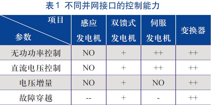
** Remarks: ++ means excellent Capacity, + means good capacity, - means a small amount of capacity, -- means very little capacity, NO means no such situation At present, DG is mainly based on wind power and photovoltaic power generation. Based on DG grid-connected technology, this paper focuses on the research on the reactive power characteristics of doubly-fed wind power generation system and photovoltaic power generation system. **

1.1

Power characteristics of doubly-fed wind turbine

Reactive power characteristics of doubly-fed wind turbine are affected by stator winding, rotor winding and rotor Influenced by factors such as side current [13], the maximum value of rotor side current plays a major role in the reactive power operating range. The reactive power output of the grid-side converter can in principle be controlled independently of the real power output, but does not exceed the apparent power.

Under the constraint conditions, the relationship between the maximum reactive output power Qmax of the wind turbine, the active power P, and the maximum apparent power Smax is shown in formula (1):

The mechanical and electrical characteristics of a doubly-fed wind turbine largely depend on the slip The active power of the rotor is proportional to the slip. Therefore, the reactive power capacity of the wind turbine also depends on the slip, and the formula (1) can be simplified as:

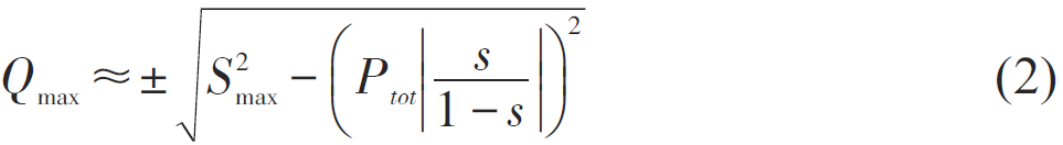
In the formula, s is the slip ratio of the stator and rotor of the wind turbine, Ptot is the total power, and it means that the total power is limited by the slip ratio.

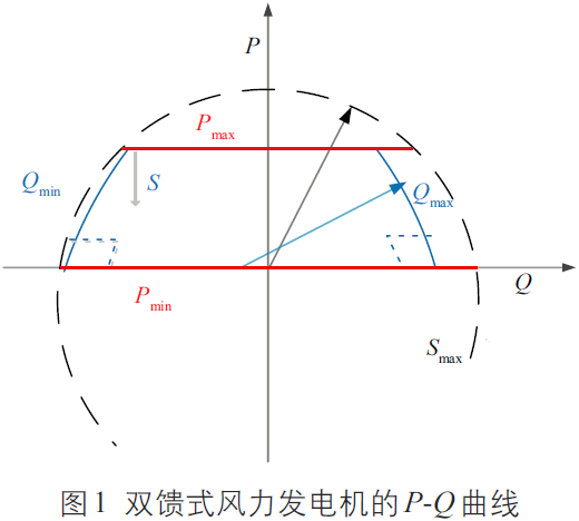
The total power of a wind turbine is the sum of the stator power and the effective rotor power. The slip rate is limited by the rotor voltage, so the slip rate will not be too high, and the reactive power Qmax will be further reduced.

From this, the PQ curve of the doubly-fed wind turbine can be obtained, as shown in Figure 1.

1.2

Photovoltaic power generation system Power characteristics

The grid-connected photovoltaic system can inject active power or reactive power into the grid, and the voltage relationship after being integrated into the grid is:

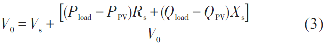
In the formula, PPV and QPV are the active power and reactive power injected into the grid by the photovoltaic system respectively; Pload and Qload are respectively Active power and reactive power of the load; V0 is the initial voltage; Vs is the calculated voltage; Rs is the photovoltaic system resistance; Xs is the photovoltaic system reactance.

When the incremental change of △u occurs at the grid-connected point voltage, the corresponding incremental change of △i occurs, then:

In the formula, ΔPPV is the variation of active power of the photovoltaic system; ΔIQ is the variation of reactive current of the photovoltaic system; φ is the equivalent impedance angle; θ is the power factor angle of the photovoltaic grid-connected system; Sk is the apparent power. The constraints on the reactive power generated by the inverter are:

< /p>

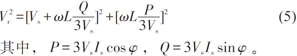
In the formula, Vr is the output voltage of the inverter; Vs is the input voltage of the inverter; ω is the phase rotation speed; L is the inductance of the photovoltaic system; P is the active power of the photovoltaic system; System reactive power; Is is input current. The reactive power constraints of the system are:

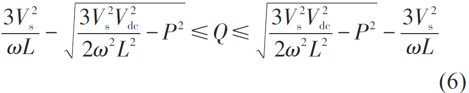
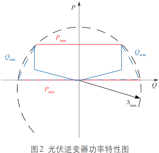
In the formula, Vdc is the DC input voltage. The inverter capacity constraints are:

In the formula, S is the apparent power of the inverter. From this, the photovoltaic power characteristic diagram can be obtained, as shown in Figure 2.

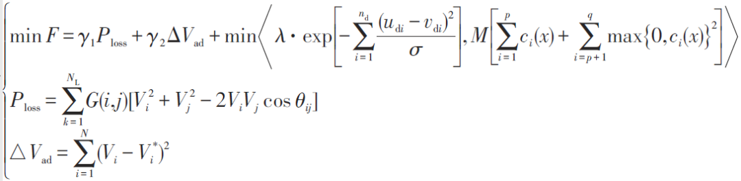
In the formula, F is the objective function; Ploss is the active power loss; △Vad is the voltage increment of node i, V * i is the reference voltage of node i; γ1 and γ2 are distribution coefficients. The power flow constraints are:

Two

Mathematical model for active distribution network reactive power optimization

Under the premise of comprehensively considering the reliability and economy of the system in the active distribution network, the coordinated control of active power and reactive power is self-regulated through the priority DG. Considering the global optimality of the active distribution network, this paper takes the active network loss and system voltage offset as the reactive power optimization index, and uses the method of fixed weight to transform the multi-objective optimization problem into a single-objective optimization problem, considering the system node The voltage and reactive power output of the generator are prone to cross-border situations, and the Gaussian penalty function is introduced to construct the model, as shown in formula (9).

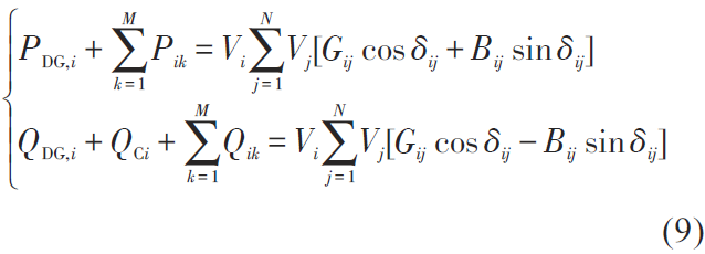
** In the formula, PDG,i, QDG, i are the active power and reactive power injected into the grid by node i respectively; Pik and Qik are the active power and reactive power output by the kth generator set at node i respectively; Vi and Vj are the voltage amplitudes of nodes i and j respectively ; θij is the voltage phase angle difference; **

Gij and Bij are the conductance and susceptance of the line respectively; N is the number of nodes; δij is the phase angle difference of the line; QCi is the reactive power compensation of node i;

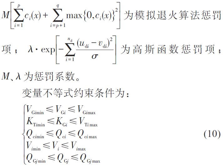
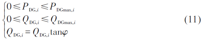
In the formula, VGi is the i-node injection Voltage; KTi is power frequency; Qci is the compensation capacity of shunt capacitor; Vi is the voltage of node i; QGj is the reactive power injected by node j. DG running constraints are:

< strong>Three

Solution of simulated annealing penalty function

In this paper, the Gaussian penalty function is introduced into the control strategy of the original dual interior point method, To achieve continuous discrete variables; compared with discontinuous penalty functions, Gaussian penalty functions have continuous differentiable advantages; and simulated annealing penalty functions [14-16] can avoid falling into local optimum in Gaussian penalty functions, so as to achieve global optimize.

Therefore, this paper proposes a strategy combining stepwise warping with parametric testing [17]. Based on the Gaussian penalty function method, the simulated annealing penalty function method and the primal dual interior point method, a practical algorithm for solving discrete variable reactive power optimization problems is designed. The selection of relevant parameters is as follows: Fmin represents the optimal solution of the objective function obtained by the continuous process of each variable; initial penalty coefficient λ0 =10-5Fmin; M=105; neighborhood size factor σ =0.25nd. During the solution process, the discrete control variable is divided into a slack part and a fixed part. The slack part refers to the continuous discrete variable, and its index set is expressed as Islack; the fixed part refers to the warped discrete variable, and its index set is expressed as Ifix.

The designed algorithm steps are as follows:

1) Initialize the interior point method [18-21], set λ = 0, and ignore the discrete control variables The penalty function is not warped. The optimal solution (x*,uc,ud)T and the optimal target Fmin of each variable in the continuous process are obtained.

2) Set k =1, ν(k -1) =10-5Fmin, the range of integer ud is [U- ] d, Uˉd, and calculate the neighborhood center vdi =|u | di +0.5, set the neighborhood size factor σ =0.25nd, the warping threshold is δ, the penalty coefficient growth factor β =2.5, the iteration initial value (x(0),u(0)c ,u( 0) d ) = (x*,u*c,u*d)T .

3) Set (x(k),u(k)c ,u(k)d )=(x(k -1),u(k -1)c ,u(k - 1)d )T , it can be used as the initial value of iteration. Use the Gaussian penalty function and the original dual interior point method to solve the optimal problem with the penalty term, and start the simulated annealing penalty term at the same time, compare the Gaussian penalty function and the simulated annealing penalty function to take the optimal value, and obtain (x(k),u(k )c ,u(k)d )=(x(k 1),u(k -1)c ,u(k -1)d )T the optimal solution.

4) Search each component u(k)di of the discrete variable u(k)d and classify it. If u(k)di ≤ -Ud +δ, then i ∈ Ifix, u(k)di = -Ud, if u(k)di ≤ -Ud -δ, set i ∈ Ifix, u(k)di = Uˉd ; otherwise set i ∈ Islack.

1. If there is no new range lower limit Ifix, set λ(k) =βλ(k -1)(β＞1), otherwise set λ(k) =λ0.

6) If Ifix =nd, then skip to step 7); otherwise, set k =k +1, and skip to step 3).

7) Verify the optimal solution (x*,uc,ud)T and the optimal target Fmin, and output the result.

The calculation steps of the simulated annealing penalty item are:

1. Set the range of the initial variable range integer u*d to [U- ] d, Uˉd , randomly select the initial state x0, and calculate the simulated annealing penalty item p(x0).

2. Select xr1, xr2,...,xrm rotation variables, △p(x)=p(x)-p(x0).

3) Under the temperature parameter T, repeat steps 2) and 3) for a certain number of times.

4) Gradually cool down, Tk +1 = αTk, 0<α<1.

5) Repeat step 2), step 5) until convergence.

Fourth

Example

Based on the IEEE 14-node distribution system, the power distribution The 3 transformers in the system are equipped with on-load voltage regulating transformers; 3 DGs and 2 groups of parallel capacitors are added; the line parameters and load parameters remain unchanged. The ratio range of the compensation capacity of the shunt capacitor to the underload voltage dividing capacity (ULTC) is 0.91.1, which can be divided into 8 levels with a step size of 0.025. Assume that DG1 and DG2 are photovoltaic power sources with a certain reactive capacity, which are connected to node 10 and node 13 respectively. For each photovoltaic DG, the apparent power Sg = 0.033pu, the active power output Pg = 0.03pu; DG3 is a doubly-fed wind generator with a certain reactive capacity, and connected to 4 nodes, its apparent power Sg = 0.4pu, active power Pg =0.3pu. The reactive power of each DG satisfies the reactive constraint equation. The gears of the two sets of parallel capacitors are 0.06pu ×(-14) and 0.05pu ×(18) respectively, and the voltage range of all P and Q points is 0.951.05pu, The voltage range of photovoltaic nodes is 0.9~1.1pu.

The optimal solutions of reactive power optimization results under different penalty functions are shown in Table 2. The optimal solutions of the interior point-Gauss method and interior point-annealing method in Table 2 refer to the values of all variables in the continuous process The optimal value. Comparing before optimization and after optimization, the net loss of the whole system dropped from 13.39MW to 9.35MW, a drop of 30.17%. The voltage of each node fluctuates less within the constraints. Therefore, using the reactive power compensation capability of DG can provide good support for the grid voltage and greatly reduce energy loss.

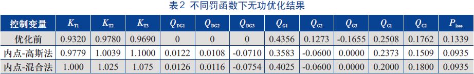
From Table 2, the data power loss is reduced from 0.1339 To 0.0935, through comparison, it can be found that the limited penalty function iteration is optimized by the annealing method, so that the Gaussian method can jump out of the local optimum, and then achieve reactive power optimization, and finally achieve the goal of minimizing the system active power loss.

According to the optimization theory, the optimal value of the introduced penalty function is greater than or equal to the optimal value of the original continuous problem, and the simulated annealing penalty function is introduced in the penalty function processing to prevent the Gaussian penalty function from falling into a local optimum. From this perspective, the penalty function improves the feasibility of the relaxed solution while maintaining the compromise of the optimal solution. In the control formula of the reactive local control scheme, according to the purpose of DG participating in the auxiliary service of the grid, some losses are adjusted to maintain local voltage stability or provide sufficient reactive power for the power system.

Five

Conclusion

1) The introduction of the Gaussian penalty function method in this paper not only keeps the optimization The continuity of , and the optimal result is normalized, which can be effectively applied to the problem of reactive power optimization discrete variable rounding.

2) In this paper, the simulated annealing penalty function is introduced in the objective function, which can not only improve the convergence accuracy and speed of the algorithm, but also effectively solve the problem that the objective function only contains the Gaussian penalty function algorithm, which causes the algorithm to fall into local optimum. obtain the global optimal result.